Entropy (information theory)
In information theory, entropy is a measure of the uncertainty associated with a random variable. In this context, the term usually refers to the Shannon entropy, which quantifies the expected value of the information contained in a message, usually in units such as bits. In this context, a 'message' means a specific realization of the random variable.
Equivalently, the Shannon entropy is a measure of the average information content one is missing when one does not know the value of the random variable. The concept was introduced by Claude E. Shannon in his 1948 paper "A Mathematical Theory of Communication".
Shannon's entropy represents an absolute limit on the best possible lossless compression of any communication, under certain constraints: treating messages to be encoded as a sequence of independent and identically-distributed random variables, Shannon's source coding theorem shows that, in the limit, the average length of the shortest possible representation to encode the messages in a given alphabet is their entropy divided by the logarithm of the number of symbols in the target alphabet.
A single toss of a fair coin has an entropy of one bit. Two tosses has an entropy of two bits. The entropy rate for the coin is one bit per toss. However, if the coin is not fair, then the uncertainty is lower (if asked to bet on the next outcome, we would bet preferentially on the most frequent result), and thus the Shannon entropy is lower. Mathematically, a single coin flip (fair or not) is an example of a Bernoulli trial, and its entropy is given by the binary entropy function. A series of tosses of a two-headed coin will have zero entropy, since the outcomes are entirely predictable. The entropy rate of English text is between 1.0 and 1.5 bits per letter,[1] or as low as 0.6 to 1.3 bits per letter, according to estimates by Shannon based on human experiments.[2]
Contents |
Introduction
Entropy is a measure of disorder, or more precisely unpredictability. For example, a series of coin tosses with a fair coin has maximum entropy, since there is no way to predict what will come next. A string of coin tosses with a coin with two heads and no tails has zero entropy, since the coin will always come up heads. Most collections of data in the real world lie somewhere in between. It is important to realize the difference between the entropy of a set of possible outcomes, and the entropy of a particular outcome. A single toss of a fair coin has an entropy of one bit, but a particular result (e.g. "heads") has zero entropy, since it is entirely "predictable".
English text has fairly low entropy. In other words, it is fairly predictable. Even if we don't know exactly what is going to come next, we can be fairly certain that, for example, there will be many more e's than z's, or that the combination 'qu' will be much more common than any other combination with a 'q' in it and the combination 'th' will be more common than any of them. Uncompressed, English text has about one bit of entropy for each byte (eight bits) of message.
If a compression scheme is lossless—that is, you can always recover the entire original message by uncompressing—then a compressed message has the same total entropy as the original, but in fewer bits. That is, it has more entropy per bit. This means a compressed message is more unpredictable, which is why messages are often compressed before being encrypted. Shannon's source coding theorem says (roughly) that a lossless compression scheme cannot compress messages, on average, to have more than one bit of entropy per bit of message. The entropy of a message is in a certain sense a measure of how much information it really contains.
Shannon's theorem also implies that no lossless compression scheme can compress all messages. If some messages come out smaller, at least one must come out larger. In the real world, this is not a problem, because we are generally only interested in compressing certain messages, for example English documents as opposed to random bytes, or digital photographs rather than noise, and don't care if our compressor makes random messages larger.
Definition
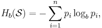
Named after Boltzmann's H-theorem, Shannon denoted the entropy H of a discrete random variable X with possible values {x1, ..., xn} as,
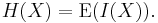
Here E is the expected value, and I is the information content of X.
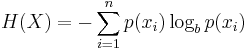
I(X) is itself a random variable. If p denotes the probability mass function of X then the entropy can explicitly be written as

where b is the base of the logarithm used. Common values of b are 2, Euler's number e, and 10, and the unit of entropy is bit for b = 2, nat for b = e, and dit (or digit) for b = 10.[3]
In the case of pi = 0 for some i, the value of the corresponding summand 0 logb 0 is taken to be 0, which is consistent with the limit:
 .
.
The proof of this limit can be quickly obtained applying l'Hôpital's rule.
Example
Consider tossing a coin with known, not necessarily fair, probabilities of coming up heads or tails.
The entropy of the unknown result of the next toss of the coin is maximized if the coin is fair (that is, if heads and tails both have equal probability 1/2). This is the situation of maximum uncertainty as it is most difficult to predict the outcome of the next toss; the result of each toss of the coin delivers a full 1 bit of information.
However, if we know the coin is not fair, but comes up heads or tails with probabilities p and q, then there is less uncertainty. Every time it is tossed, one side is more likely to come up than the other. The reduced uncertainty is quantified in a lower entropy: on average each toss of the coin delivers less than a full 1 bit of information.
The extreme case is that of a double-headed coin that never comes up tails, or a double-tailed coin that never results in a head. Then there is no uncertainty. The entropy is zero: each toss of the coin delivers no information.
Rationale
For a random variable  with
with  outcomes
  , the Shannon entropy, a measure of uncertainty (see further below) and denoted by
  , is defined as
-
(1)
where  is the probability mass function of outcome
  .
.
To understand the meaning of Eq. (1), first consider a set of possible outcomes (events)  , with equal probability
  . An example would be a fair die with values, from
  to . The uncertainty for such a set of outcomes is defined by
-
(2)
The logarithm is used to provide the additivity characteristic for independent uncertainty. For example, consider appending to each value of the first die the value of a second die, which has  possible outcomes
  . There are thus
  possible outcomes
  . The uncertainty for such a set of outcomes is then
-

(3)
Thus the uncertainty of playing with two dice is obtained by adding the uncertainty of the second die  to the uncertainty of the first die
  .
.
Now return to the case of playing with one die only (the first one). Since the probability of each event is  , we can write
In the case of a non-uniform probability mass function (or density in the case of continuous random variables), we let
-
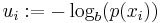
(4)
which is also called a surprisal; the lower the probability , i.e.  , the higher the uncertainty or the surprise, i.e.
  , for the outcome .
The average uncertainty  , with
  being the average operator, is obtained by
-
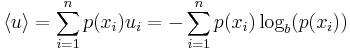
(5)
and is used as the definition of the entropy in Eq. (1). The above also explained why information entropy and information uncertainty can be used interchangeably.[4]
One may also define the conditional entropy of two events X and Y taking values xi and yj respectively, as
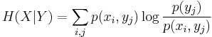
where p(xi,yj) is the probability that X=xi and Y=yj. This quantity should be understood as the amount of randomness in the random variable X given that you know the value of Y. For example, the entropy associated with a six-sided die is H(die), but if you were told that it had in fact landed on 1, 2, or 3, then its entropy would be equal to H(die: the die landed on 1, 2, or 3).
Aspects
Relationship to thermodynamic entropy
The inspiration for adopting the word entropy in information theory came from the close resemblance between Shannon's formula and very similar known formulae from thermodynamics.
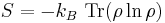
In statistical thermodynamics the most general formula for the thermodynamic entropy S of a thermodynamic system is the Gibbs entropy,
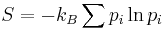
where kB is the Boltzmann constant, and pi is the probability of a microstate. The Gibbs entropy was defined by J. Willard Gibbs in 1878 after earlier work by Boltzmann (1872).[5]
The Gibbs entropy translates over almost unchanged into the world of quantum physics to give the von Neumann entropy, introduced by John von Neumann in 1927,
where ρ is the density matrix of the quantum mechanical system and Tr is the trace.
At an everyday practical level the links between information entropy and thermodynamic entropy are not evident. Physicists and chemists are apt to be more interested in changes in entropy as a system spontaneously evolves away from its initial conditions, in accordance with the second law of thermodynamics, rather than an unchanging probability distribution. And, as the minuteness of Boltzmann's constant kB indicates, the changes in S / kB for even tiny amounts of substances in chemical and physical processes represent amounts of entropy which are so large as to be off the scale compared to anything seen in data compression or signal processing. Furthermore, in classical thermodynamics the entropy is defined in terms of macroscopic measurements and makes no reference to any probability distribution, which is central to the definition of information entropy.
But, at a multidisciplinary level, connections can be made between thermodynamic and informational entropy, although it took many years in the development of the theories of statistical mechanics and information theory to make the relationship fully apparent. In fact, in the view of Jaynes (1957), thermodynamic entropy, as explained by statistical mechanics, should be seen as an application of Shannon's information theory: the thermodynamic entropy is interpreted as being proportional to the amount of further Shannon information needed to define the detailed microscopic state of the system, that remains uncommunicated by a description solely in terms of the macroscopic variables of classical thermodynamics, with the constant of proportionality being just the Boltzmann constant. For example, adding heat to a system increases its thermodynamic entropy because it increases the number of possible microscopic states for the system, thus making any complete state description longer. (See article: maximum entropy thermodynamics). Maxwell's demon can (hypothetically) reduce the thermodynamic entropy of a system by using information about the states of individual molecules; but, as Landauer (from 1961) and co-workers have shown, to function the demon himself must increase thermodynamic entropy in the process, by at least the amount of Shannon information he proposes to first acquire and store; and so the total thermodynamic entropy does not decrease (which resolves the paradox).
Entropy as information content
Entropy is defined in the context of a probabilistic model. Independent fair coin flips have an entropy of 1 bit per flip. A source that always generates a long string of B's has an entropy of 0, since the next character will always be a 'B'.
The entropy rate of a data source means the average number of bits per symbol needed to encode it. Shannon's experiments with human predictors show an information rate of between 0.6 and 1.3 bits per character,[6] depending on the experimental setup; the PPM compression algorithm can achieve a compression ratio of 1.5 bits per character in English text.
From the preceding example, note the following points:
- The amount of entropy is not always an integer number of bits.
- Many data bits may not convey information. For example, data structures often store information redundantly, or have identical sections regardless of the information in the data structure.
Shannon's definition of entropy, when applied to an information source, can determine the minimum channel capacity required to reliably transmit the source as encoded binary digits (see caveat below in italics). The formula can be derived by calculating the mathematical expectation of the amount of information contained in a digit from the information source. See also Shannon-Hartley theorem.
Shannon's entropy measures the information contained in a message as opposed to the portion of the message that is determined (or predictable). Examples of the latter include redundancy in language structure or statistical properties relating to the occurrence frequencies of letter or word pairs, triplets etc. See Markov chain.
Data compression
Entropy effectively bounds the performance of the strongest lossless (or nearly lossless) compression possible, which can be realized in theory by using the typical set or in practice using Huffman, Lempel-Ziv or arithmetic coding. The performance of existing data compression algorithms is often used as a rough estimate of the entropy of a block of data.[7][8] See also Kolmogorov complexity.
Limitations of entropy as information content
There are a number of entropy-related concepts that mathematically quantify information content in some way:
- the self-information of an individual message or symbol taken from a given probability distribution,
- the entropy of a given probability distribution of messages or symbols, and
- the entropy rate of a stochastic process.
(The "rate of self-information" can also be defined for a particular sequence of messages or symbols generated by a given stochastic process: this will always be equal to the entropy rate in the case of a stationary process.) Other quantities of information are also used to compare or relate different sources of information.
It is important not to confuse the above concepts. Oftentimes it is only clear from context which one is meant. For example, when someone says that the "entropy" of the English language is about 1.5 bits per character, they are actually modeling the English language as a stochastic process and talking about its entropy rate.
Although entropy is often used as a characterization of the information content of a data source, this information content is not absolute: it depends crucially on the probabilistic model. A source that always generates the same symbol has an entropy rate of 0, but the definition of what a symbol is depends on the alphabet. Consider a source that produces the string ABABABABAB... in which A is always followed by B and vice versa. If the probabilistic model considers individual letters as independent, the entropy rate of the sequence is 1 bit per character. But if the sequence is considered as "AB AB AB AB AB..." with symbols as two-character blocks, then the entropy rate is 0 bits per character.
However, if we use very large blocks, then the estimate of per-character entropy rate may become artificially low. This is because in reality, the probability distribution of the sequence is not knowable exactly; it is only an estimate. For example, suppose one considers the text of every book ever published as a sequence, with each symbol being the text of a complete book. If there are N published books, and each book is only published once, the estimate of the probability of each book is 1/N, and the entropy (in bits) is -log2 1/N = log2 N. As a practical code, this corresponds to assigning each book a unique identifier and using it in place of the text of the book whenever one wants to refer to the book. This is enormously useful for talking about books, but it is not so useful for characterizing the information content of an individual book, or of language in general: it is not possible to reconstruct the book from its identifier without knowing the probability distribution, that is, the complete text of all the books. The key idea is that the complexity of the probabilistic model must be considered. Kolmogorov complexity is a theoretical generalization of this idea that allows the consideration of the information content of a sequence independent of any particular probability model; it considers the shortest program for a universal computer that outputs the sequence. A code that achieves the entropy rate of a sequence for a given model, plus the codebook (i.e. the probabilistic model), is one such program, but it may not be the shortest.
For example, the Fibonacci sequence is 1, 1, 2, 3, 5, 8, 13, ... . Treating the sequence as a message and each number as a symbol, there are almost as many symbols as there are characters in the message, giving an entropy of approximately log2(n). So the first 128 symbols of the Fibonacci sequence has an entropy of approximately 7 bits/symbol. However, the sequence can be expressed using a formula [F(n) = F(n-1) + F(n-2) for n={3,4,5,...}, F(1)=1, F(2)=1] and this formula has a much lower entropy and applies to any length of the Fibonacci sequence.
Limitations of entropy as a measure of unpredictability
In cryptanalysis, entropy is often roughly used as a measure of the unpredictability of a cryptographic key. For example, a 128-bit key that is randomly generated has 128 bits of entropy. It takes (on average)  guesses to break by brute force. If the key's first digit is 0, and the others random, then the entropy is 127 bits, and it takes (on average)
  guesses.
However, this measure fails if the possible keys are not of equal probability. If the key is half the time "password" and half the time a true random 128-bit key, then the entropy is approximately 65 bits. Yet half the time the key may be guessed on the first try, if your first guess is "password", and on average, it takes around  guesses (not
  ) to break this password.
Similarly, consider a 1000000-digit binary one-time pad. If the pad has 1000000 bits of entropy, it is perfect. If the pad has 999999 bits of entropy, evenly distributed (each individual bit of the pad having 0.999999 bits of entropy) it may still be considered very good. But if the pad has 999999 bits of entropy, where the first digit is fixed and the remaining 999999 digits are perfectly random, then the first digit of the ciphertext will not be encrypted at all.
Data as a Markov process
A common way to define entropy for text is based on the Markov model of text. For an order-0 source (each character is selected independent of the last characters), the binary entropy is:
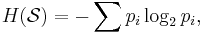
where pi is the probability of i. For a first-order Markov source (one in which the probability of selecting a character is dependent only on the immediately preceding character), the entropy rate is:
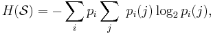
where i is a state (certain preceding characters) and  is the probability of
  given
given  as the previous character.
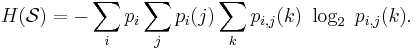
For a second order Markov source, the entropy rate is
b-ary entropy
In general the b-ary entropy of a source  = (S,P) with source alphabet S = {a1, ..., an} and discrete probability distribution P = {p1, ..., pn} where pi is the probability of ai (say pi = p(ai)) is defined by:
Note: the b in "b-ary entropy" is the number of different symbols of the "ideal alphabet" which is being used as the standard yardstick to measure source alphabets. In information theory, two symbols are necessary and sufficient for an alphabet to be able to encode information, therefore the default is to let b = 2 ("binary entropy"). Thus, the entropy of the source alphabet, with its given empiric probability distribution, is a number equal to the number (possibly fractional) of symbols of the "ideal alphabet", with an optimal probability distribution, necessary to encode for each symbol of the source alphabet. Also note that "optimal probability distribution" here means a uniform distribution: a source alphabet with n symbols has the highest possible entropy (for an alphabet with n symbols) when the probability distribution of the alphabet is uniform. This optimal entropy turns out to be  .
.
Efficiency
A source alphabet with non-uniform distribution will have less entropy than if those symbols had uniform distribution (i.e. the "optimized alphabet"). This deficiency in entropy can be expressed as a ratio:
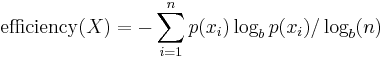
Efficiency has utility in quantifying the effective use of a communications channel.
Characterization
Shannon entropy is characterized by a small number of criteria, listed below. Any definition of entropy satisfying these assumptions has the form
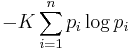
where K is a constant corresponding to a choice of measurement units.
In the following, 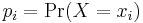 and
and  .
.
Continuity
The measure should be continuous, so that changing the values of the probabilities by a very small amount should only change the entropy by a small amount.
Symmetry
The measure should be unchanged if the outcomes xi are re-ordered.
 etc.
etc.
Maximum
The measure should be maximal if all the outcomes are equally likely (uncertainty is highest when all possible events are equiprobable).
For equiprobable events the entropy should increase with the number of outcomes.
Additivity
The amount of entropy should be independent of how the process is regarded as being divided into parts.
This last functional relationship characterizes the entropy of a system with sub-systems. It demands that the entropy of a system can be calculated from the entropies of its sub-systems if the interactions between the sub-systems are known.
Given an ensemble of n uniformly distributed elements that are divided into k boxes (sub-systems) with b1, b2, ... , bk elements each, the entropy of the whole ensemble should be equal to the sum of the entropy of the system of boxes and the individual entropies of the boxes, each weighted with the probability of being in that particular box.
For positive integers bi where b1 + ... + bk = n,
Choosing k = n, b1 = ... = bn = 1 this implies that the entropy of a certain outcome is zero:

This implies that the efficiency of a source alphabet with n symbols can be defined simply as being equal to its n-ary entropy. See also Redundancy (information theory).
Further properties
The Shannon entropy satisfies the following properties, for some of which it is useful to interpret entropy as the amount of information learned (or uncertainty eliminated) by revealing the value of a random variable X:
- Adding or removing an event with probability zero does not contribute to the entropy:
 .
.
- It can be confirmed using the Jensen inequality that
![H(X) = \operatorname{E}\left[\log_b \left( \frac{1}{p(X)}\right) \right]
\leq \log_b \left[ \operatorname{E}\left( \frac{1}{p(X)} \right) \right]
= \log_b(n)](/2012-wikipedia_en_all_nopic_01_2012/I/4fbd45c6f6a42adfb9be446fde37a341.png) .
.
This maximal entropy of  is effectively attained by a source alphabet having a uniform probability distribution: uncertainty is maximal when all possible events are equiprobable.
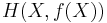
- The entropy or the amount of information revealed by evaluating (X,Y) (that is, evaluating X and Y simultaneously) is equal to the information revealed by conducting two consecutive experiments: first evaluating the value of Y, then revealing the value of X given that you know the value of Y. This may be written as
![H[(X,Y)]=H(X|Y)%2BH(Y).](/2012-wikipedia_en_all_nopic_01_2012/I/57739b0d57213bf3b4f0880b8f316b1c.png)
- If Y=f(X) where f is deterministic, then applying the previous formula to
 yields
 so
so 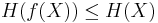 ,
,
thus the entropy of a variable can only decrease when the latter is passed through a deterministic function.
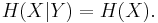
- If X and Y are two independent experiments, then knowing the value of Y doesn't influence our knowledge of the value of X (since the two don't influence each other by independence):
- The entropy of two simultaneous events is no more than the sum of the entropies of each individual event, and are equal if the two events are independent. More specifically, if X and Y are two random variables on the same probability space, and (X,Y) denotes their Cartesian product, then
![H[(X,Y)]\leq H(X)%2BH(Y).](/2012-wikipedia_en_all_nopic_01_2012/I/3a4d0c6ba32f90befe93ee8362587811.png)
Proving this mathematically follows easily from the previous two properties of entropy.
Extending discrete entropy to the continuous case: differential entropy
The Shannon entropy is restricted to random variables taking discrete values. The formula
![h[f] = -\int\limits_{-\infty}^{\infty} f(x) \log f(x)\, dx,\quad (1)](/2012-wikipedia_en_all_nopic_01_2012/I/98c89b631013dd10b7183323ddb8c9fb.png)
where f denotes a probability density function on the real line, is analogous to the Shannon entropy and could thus be viewed as an extension of the Shannon entropy to the domain of real numbers.
A precursor of the continuous entropy ![h[f]](/2012-wikipedia_en_all_nopic_01_2012/I/7eeba783ae7085af07e0e88e3fbe1cfb.png) given in (1) is the expression for the functional
given in (1) is the expression for the functional  in the H-theorem of Boltzmann.
Formula (1) is usually referred to as the continuous entropy, or differential entropy. Although the analogy between both functions is suggestive, the following question must be set: is the differential entropy a valid extension of the Shannon discrete entropy? Differential entropy lacks a number of properties that the Shannon discrete entropy has – it can even be negative – and thus corrections have been suggested, notably limiting density of discrete points.
To answer this question, we must establish a connection between the two functions:
We wish to obtain a generally finite measure as the bin size goes to zero. In the discrete case, the bin size is the (implicit) width of each of the n (finite or infinite) bins whose probabilities are denoted by pn. As we generalize to the continuous domain, we must make this width explicit.
To do this, start with a continuous function f discretized as shown in the figure. As the figure indicates, by the mean-value theorem there exists a value xi in each bin such that
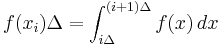
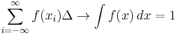
and thus the integral of the function f can be approximated (in the Riemannian sense) by
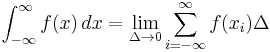
where this limit and "bin size goes to zero" are equivalent.
We will denote

and expanding the logarithm, we have
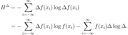
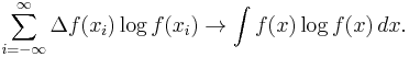
As  , we have
and also
But note that  as , therefore we need a special definition of the differential or continuous entropy:
![h[f] = \lim_{\Delta \to 0} \left[H^{\Delta} %2B \log \Delta\right] = -\int_{-\infty}^{\infty} f(x) \log f(x)\,dx,](/2012-wikipedia_en_all_nopic_01_2012/I/8bee995e9adc878eb0810576e299b84b.png)
which is, as said before, referred to as the differential entropy. This means that the differential entropy is not a limit of the Shannon entropy for  . Rather, if differs from the limit of the Shannon entropy by an infinite offset.
It turns out as a result that, unlike the Shannon entropy, the differential entropy is not in general a good measure of uncertainty or information. For example, the differential entropy can be negative; also it is not invariant under continuous co-ordinate transformations.
Another useful measure of entropy for the continuous case is the relative entropy of a distribution, defined as the Kullback-Leibler divergence from the distribution to a reference measure m(x),
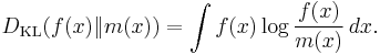
The relative entropy carries over directly from discrete to continuous distributions, is always positive or zero, and is invariant under co-ordinate reparameterizations.
Use in combinatorics
Entropy has become a useful quantity in combinatorics.
Loomis-Whitney inequality
A simple example of this is an alternate proof of the Loomis-Whitney inequality: for every subset  , we have
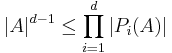
where  , that is,
  is the orthogonal projection in the ith coordinate.
The proof follows as a simple corollary of Shearer's inequality: if  are random variables and
  are subsets of
 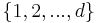 such that every integer between 1 and d lie in exactly r of these subsets, then
![H[(X_{1},...,X_{d})]\leq \frac{1}{r}\sum_{i=1}^{n}H[(X_{j})_{j\in S_{i}}]](/2012-wikipedia_en_all_nopic_01_2012/I/31a85f9c121805adfc75f3e458e049c9.png)
where  is the Cartesian product of random variables
  with indexes j in
  (so the dimension of this vector is equal to the size of ).
We sketch how Loomis-Whitney follows from this: Indeed, let X be a uniformly distributed random variable with values in A and so that each point in A occurs with equal probability. Then (by the further properties of entropy mentioned above) 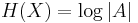 , where |A| denotes the cardinality of A. Let
  . The range of is contained in
  and hence
 ![H[(X_{j})_{j\in S_{i}}]\leq \log |P_{i}(A)|](/2012-wikipedia_en_all_nopic_01_2012/I/c8a2949b3b77933bccc24b4be6e2d3d1.png) . Now use this to bound the right side of Shearer's inequality and exponentiate the opposite sides of the resulting inequality you obtain.
. Now use this to bound the right side of Shearer's inequality and exponentiate the opposite sides of the resulting inequality you obtain.
Approximation to binomial coefficient
For integers  let
let  . Then
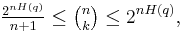
where  .[9]
.[9]
Here is a sketch proof. Note that 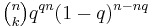 is one term of the expression
 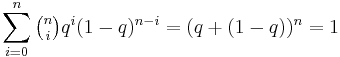 . Rearranging gives the upper bound. For the lower bound one first shows, using some algebra, that it is the largest term in the summation. But then,
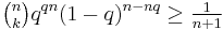
since there are  terms in the summation. Rearranging gives the lower bound.
A nice interpretation of this is that the number of binary strings of length  with exactly
  many 1's is approximately
  .[10]
.[10]
See also
- Conditional entropy
- Cross entropy – is a measure of the average number of bits needed to identify an event from a set of possibilities between two probability distributions
- Entropy (arrow of time)
- Entropy encoding – a coding scheme that assigns codes to symbols so as to match code lengths with the probabilities of the symbols.
- Entropy estimation
- Entropy power inequality
- Entropy rate
- Fisher information
- Hamming distance
- History of entropy
- History of information theory
- Joint entropy – is the measure how much entropy is contained in a joint system of two random variables.
- Kolmogorov-Sinai entropy in dynamical systems
- Levenshtein distance
- Mutual information
- Negentropy
- Perplexity
- Qualitative variation – other measures of statistical dispersion for nominal distributions
- Quantum relative entropy – a measure of distinguishability between two quantum states.
- Rényi entropy – a generalisation of Shannon entropy; it is one of a family of functionals for quantifying the diversity, uncertainty or randomness of a system.
- Shannon index
- Theil index
References
- ^ Schneier, B: Applied Cryptography, Second edition, page 234. John Wiley and Sons.
- ^ Shannon, Claude E.: Prediction and entropy of printed English, The Bell System Technical Journal, 30:50–64, January 1951.
- ^ Schneider, T.D, Information theory primer with an appendix on logarithms, National Cancer Institute, 14 April 2007.
- ^ Jaynes, E.T. (May 1957). "Information Theory and Statistical Mechanics". Physical Review 106 (4): 620–630. Bibcode 1957PhRv..106..620J. doi:10.1103/PhysRev.106.620. http://bayes.wustl.edu/etj/articles/theory.1.pdf.
- ^ Compare: Boltzmann, Ludwig (1896, 1898). Vorlesungen über Gastheorie : 2 Volumes – Leipzig 1895/98 UB: O 5262-6. English version: Lectures on gas theory. Translated by Stephen G. Brush (1964) Berkeley: University of California Press; (1995) New York: Dover ISBN 0-486-68455-5
- ^ Mark Nelson (2006-08-24). "The Hutter Prize". http://marknelson.us/2006/08/24/the-hutter-prize/. Retrieved 2008-11-27.
- ^ T. Schürmann and P. Grassberger, Entropy Estimation of Symbol Sequences, CHAOS,Vol. 6, No. 3 (1996) 414–427
- ^ T. Schürmann, Bias Analysis in Entropy Estimation J. Phys. A: Math. Gen. 37 (2004) L295-L301.
- ^ Aoki, New Approaches to Macroeconomic Modeling. page 43.
- ^ Probability and Computing, M. Mitzenmacher and E. Upfal, Cambridge University Press
This article incorporates material from Shannon's entropy on PlanetMath, which is licensed under the Creative Commons Attribution/Share-Alike License.
External links
- Introduction to entropy and information on Principia Cybernetica Web
- Entropy an interdisciplinary journal on all aspect of the entropy concept. Open access.
- Information is not entropy, information is not uncertainty ! – a discussion of the use of the terms "information" and "entropy".
- I'm Confused: How Could Information Equal Entropy? – a similar discussion on the bionet.info-theory FAQ.
- Description of information entropy from "Tools for Thought" by Howard Rheingold
- A java applet representing Shannon's Experiment to Calculate the Entropy of English
- Slides on information gain and entropy
- An Intuitive Guide to the Concept of Entropy Arising in Various Sectors of Science – a wikibook on the interpretation of the concept of entropy.
|
||||||||||||||||||||||||||||||||||||||||||||||||||||